

EXPAND ALL
- Home
- About Pixie
- Installing Pixie
- Using Pixie
- Tutorials
- Reference

This tutorial series demonstrates how to write a PxL script to analyze the volume of traffic coming in and out of each pod in your cluster (total bytes received vs total bytes sent).
In Part 1 of this tutorial, we will write a very basic PxL script which simply queries a table of traced network connection data provided by Pixie's no-instrumentation monitoring platform.
my_first_script.pxl:touch my_first_script.pxl
1# Import Pixie's module for querying data2import px34# Load the last 30 seconds of Pixie's `conn_stats` table into a Dataframe.5df = px.DataFrame(table='conn_stats', start_time='-30s')67# Display the DataFrame with table formatting8px.display(df)
On
line 2we import Pixie'spxmodule. This is Pixie's main library for querying data.
Pixie's scripts are written using the Pixie Language (PxL), a DSL that follows the API of the the popular Python data processing library Pandas. Pandas uses DataFrames to represent tables of data.
On
line 5we load the last 30 seconds of data from theconn_statstable into a DataFrame.
The
conn_statstable contains high-level statistics about the connections (i.e. client-server pairs) that Pixie has traced in your cluster.
On
line 8we display the table usingpx.display().
px live -f my_first_script.pxl
Your CLI should output something similar to the following table:
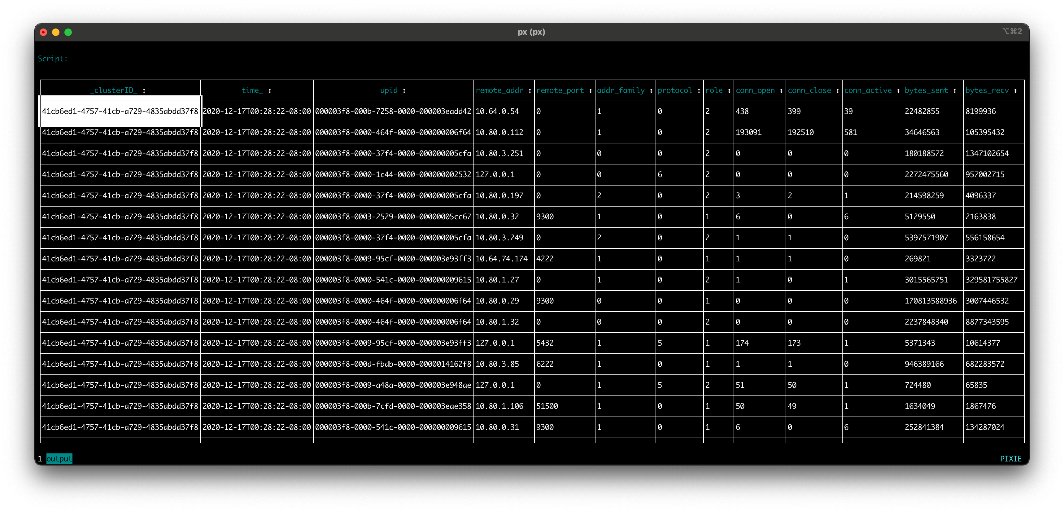
This PxL script outputs a table of data representing the last 30 seconds of the traced client-server connections in your cluster. Columns include:
time_: Timestamp when the data record was collected.upid An opaque numeric ID that globally identifies a running process inside the cluster.remote_addr: IP address of the remote endpoint.remote_port: Port of the remote endpoint.addr_family: The socket address family of the connection.protocol: The protocol of the traffic on the connections.role: The role of the process that owns the connection (client=1 or server=2).conn_open: The number of connections opened since the beginning of tracing.conn_close: The number of connections closed since the beginning of tracing.conn_active: The number of active connections.bytes_sent: The number of bytes sent to the remote endpoint(s).bytes_recv: The number of bytes received from the remote endpoint(s).You can find the conn_stats column descriptions as well as descriptions for all of the data tables provided by Pixie in the data table reference docs or by running the pre-built px/schemas script:
Exit the Live CLI using ctrl+c
Run the px/schemas script:
px live px/schemas
conn_stats in the table_name column. You should see all of the columns available in the conn_stats table listed with their descriptions.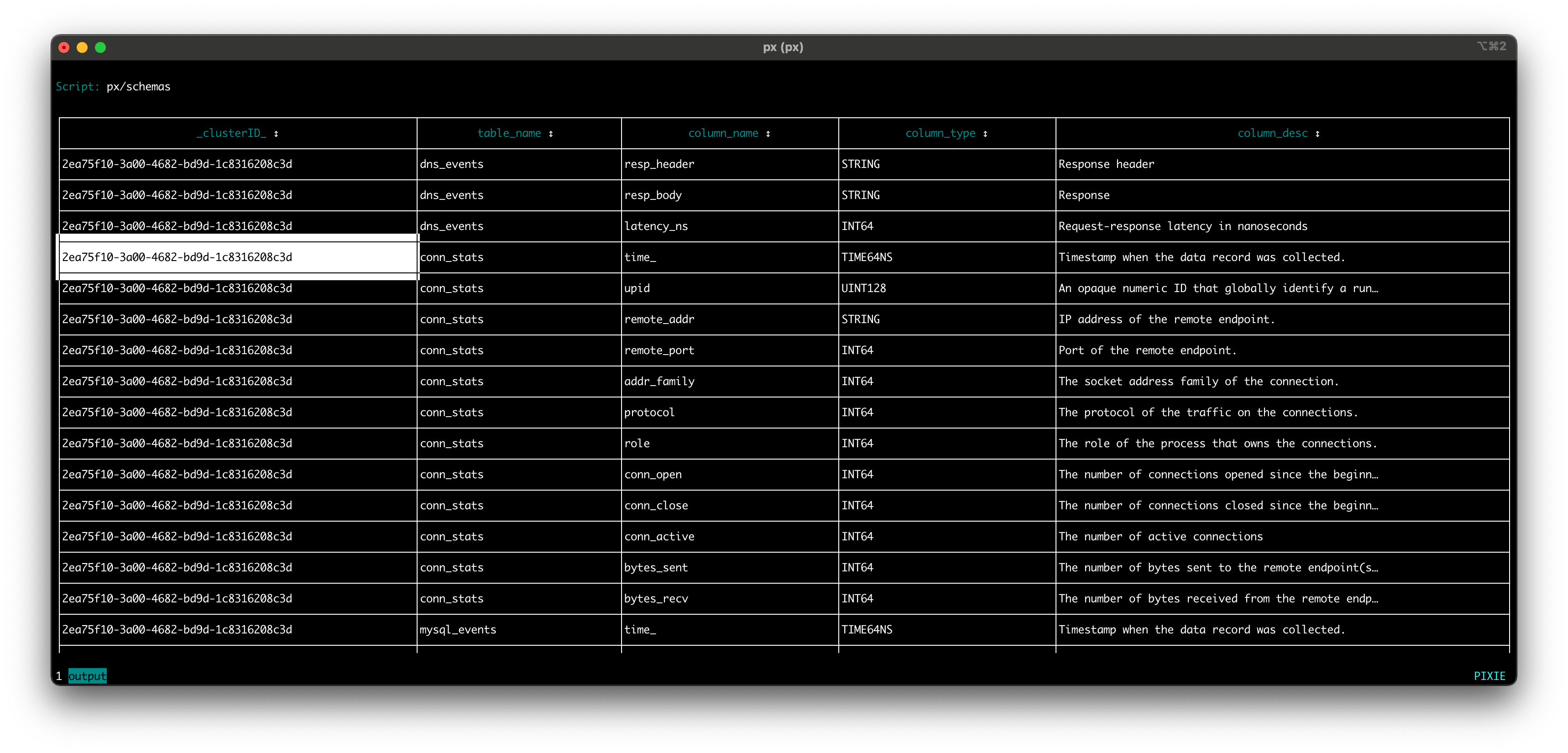
DataFrame initialization supports end_time for queries requiring more precise time periods. If an end_time isn't provided, the DataFrame will return all events up to the current time.
1import px23df = px.DataFrame(table='conn_stats', start_time='-60s', end_time='-30s')45px.display(df)
You can drop columns using the df.drop() command.
1import px23df = px.DataFrame(table='conn_stats', start_time='-30s')45# Drop select columns6df = df.drop(['conn_open', 'conn_close', 'bytes_sent', 'bytes_recv'])78px.display(df)
Alternatively, you can use keep to return a DataFrame with only the specified columns. This can be used to reorder the columns in the output.
1import px23df = px.DataFrame(table='conn_stats', start_time='-30s')45# Keep only the select columns6df = df[['remote_addr', 'conn_open', 'conn_close']]78px.display(df)
If you only need a few columns from a table, use the DataFrame's select argument instead.
1import px23# Populate the DataFrame with only the select columns from the `conn_stats` table4df = px.DataFrame(table='conn_stats', select=['remote_addr', 'conn_open', 'conn_close'], start_time='-30s')56px.display(df)
To filter the rows in the DataFrame by the role column:
1import px23df = px.DataFrame(table='conn_stats', start_time='-30s')45# Filter the results to only include rows whose `role` value equals 1 (connections traced on the client-side)6df = df[df.role == 1]78px.display(df)
If you want to see a small sample of data, you can limit the number of rows in the returned DataFrame to the first n rows (line 4).
1import px23df = px.DataFrame(table='conn_stats', start_time='-30s')45# Limit the number of rows in the DataFrame to 1006df = df.head(100)78px.display(df)
Congratulations, you built your first script!
In Tutorial #2, we will expand this PxL script to produce a table that summarizes the total amount of traffic coming in and out of each of the pods in your cluster.
This video summarizes the content in part 1 and part 2 of this tutorial:
